I’ve written several theoretical articles on world models so far — from the mathematics of RSSM to Sim-to-Real transfer, to the comparison between VLAs and world models. A reader asked: “I get the theory, but how do I actually run something?”
Today’s article answers that question. I’ll walk you step by step through setting up a complete world model experimentation environment — from installation to training to visualization. Once you’ve gotten through it, you can build your own experiments on this foundation.
Our toolchain of choice: MuJoCo (physics simulation) + DreamerV3 (world model). If you need higher-fidelity rendering, you can later switch to Isaac Sim, but MuJoCo is more than sufficient for getting started.
Tool Selection: Why These Two
MuJoCo: One of the most mainstream engines in robot simulation today. High physics accuracy, clean API, fast performance. Acquired and open-sourced for free by DeepMind in 2021, it is now the de facto standard for robot learning research and one of the most commonly used benchmarks in continuous-control world model research.
DreamerV3: A world model algorithm developed by Danijar Hafner and collaborators, the third generation of the Dreamer series. It uses RSSM (Recurrent State-Space Model) to learn environment dynamics and trains Actor-Critic policies in imagined space. The code is open-source with clear documentation, making it the best starting point for learning about world models. Note that DreamerV3 is built on the JAX + Haiku framework, not TensorFlow.
Log Format Note: DreamerV3 (commit e3f02248) outputs its own log format (metrics.jsonl and scores.jsonl), not TensorBoard event files. Despite the “json” in the name, these are JSON Lines format (one JSON object per line), which can be read and visualized directly with Python. This tutorial will show you how to analyze these logs with Python.
If your local machine has insufficient memory (below 32GB), consider using cloud resources:
- Google Colab: Free GPU, approximately 12–25GB memory, suitable for quick validation. Note that Colab sessions have time limits
- AutoDL / ModelCloud: Chinese cloud platforms with hourly billing and diverse GPU options
- AWS / GCP / Azure: On-demand GPU instances, suitable for long-running experiments
The advantage of cloud execution is no local hardware limitations; the downside is uploading and downloading data and models. For beginners, Google Colab is the most economical choice.
Step 1: Environment Setup
First, confirm your system environment. This tutorial has been verified on:
- OS: Ubuntu 22.04.5 LTS (Jammy Jellyfish), kernel 6.8.0-124-generic, x86_64 architecture. Also works with Ubuntu 20.04/22.04 other versions, macOS, and WSL2
- Python: 3.10 or 3.11 (DreamerV3 has Python version requirements)
- GPU: Optional but strongly recommended. An NVIDIA GPU can significantly accelerate training
- Memory: At least 32GB (tested: 14GB + 4GB swap still OOMs during JAX compilation). If using Google Colab or a cloud server, choose a high-memory configuration
Create a new conda environment:
conda create -n worldmodel python=3.11
conda activate worldmodel
If you have an NVIDIA GPU, you need to install JAX with CUDA support (DreamerV3’s underlying framework). The default pip install jax only installs the CPU version; GPU users need to specify explicitly:
# GPU users (CUDA 12)
pip install "jax[cuda12]"

# If you need a specific CUDA version, refer to the JAX official docs:
# https://jax.readthedocs.io/en/latest/installation.html
After installation, verify that the GPU is correctly recognized:
python -c "import jax; print(jax.devices())"
If the output includes GpuDevice(id=0), the GPU is configured correctly. If you only see CpuDevice(id=0), JAX is not using the GPU — check that your NVIDIA driver and CUDA versions match.
Step 2: Install MuJoCo
MuJoCo can now be installed directly via pip, which is much easier than before:
pip install mujoco
Verify the installation:
python -c "import mujoco; print(mujoco.__version__)"
If it outputs a version number, the installation succeeded.
If you want visual rendering (to see the 3D robot view), you also need to install a rendering backend. This is where many newcomers get stuck — especially on remote servers.
# Install rendering dependencies
pip install mujoco[extras]

# For Linux without GPU or headless servers, also install OSMesa
sudo apt-get install libosmesa6-dev
On remote servers or headless machines, you must explicitly set the rendering backend environment variable, or you’ll get GLFW errors:
# Server with NVIDIA GPU
export MUJOCO_GL=egl

# Server without GPU
export MUJOCO_GL=osmesa
Add this line to ~/.bashrc to avoid setting it every time. You can check GPU status with:
nvidia-smi
Step 3: Install DreamerV3
The official DreamerV3 code is on GitHub. It’s worth noting that DreamerV3 is not a traditional Python package — its code structure, dependency management, and entry points have changed across versions. For reproducibility, it’s recommended to pin to a specific commit:
git clone https://github.com/danijar/dreamerv3.git
cd dreamerv3

# Pin to the commit verified for this tutorial (to avoid incompatibilities from future changes)
git checkout e3f02248

pip install -r requirements.txt
Note: requirements.txt includes ale_py==0.9.0 (Atari game environment dependency), which has been delisted from PyPI. If you’re only doing MuJoCo/DM Control tasks, you can skip this package: grep -v "ale_py" requirements.txt | grep -v "autorom" | pip install -r /dev/stdin. Alternatively, manually edit requirements.txt to remove the ale_py and autorom lines before installing.
If you want to use MuJoCo environments for experiments, you also need to install DeepMind’s control library:
# DeepMind Control Suite (includes MuJoCo predefined tasks)
pip install dm-control
Note: Some tutorials online say pip install dm-control-suite — that package doesn’t exist. The correct package name is dm-control.
Understanding the Code Structure: Not a Black Box
Before running experiments, take a look at DreamerV3’s code structure so you know where the core components are. Otherwise you’re just running a black box:
dreamerv3/
-- dreamerv3/                  # Core algorithm
|   -- agent.py                # Agent main logic (Actor, Critic, world model training)
|   -- rssm.py                 # RSSM core implementation (Recurrent State-Space Model)
|   -- configs.yaml            # Hyperparameter configs (defaults, dmc_vision, dmc_proprio, atari presets)
|   -- main.py                 # Training entry point
-- embodied/                   # General framework
|   -- core/                   # Infrastructure
|   |   -- replay.py           # Experience replay buffer
|   |   -- streams.py          # Data stream processing
|   |   -- wrappers.py         # Environment wrappers
|   |   -- ...
|   -- envs/                   # Environment adapters
|   |   -- dmc.py              # DM Control (MuJoCo tasks)
|   |   -- atari.py            # Atari games
|   |   -- from_gym.py         # Gymnasium adapter
|   |   -- ...
|   -- jax/                    # JAX/Haiku implementation
|   |   -- agent.py            # JAX version Agent
|   |   -- nets.py             # Neural network definitions
|   |   -- heads.py            # Output heads (predict observations, rewards, etc.)
|   |   -- opt.py              # Optimizers
|   |   -- ...
|   -- run/                    # Training pipeline
|       -- train.py            # Training loop
|       -- parallel.py         # Parallel training
|       -- train_eval.py       # Training + evaluation
-- scores/                     # Preset benchmark scores
-- Dockerfile                  # Docker configuration
-- requirements.txt            # Python dependencies
-- baselines.yaml              # Baseline configurations
-- plot.py                     # Visualization scripts
-- README.md
Key locations:
- RSSM (Recurrent State-Space Model): Implemented in
dreamerv3/rssm.py— the core of the world model, responsible for encoding observations and predicting future states - Agent logic: In
dreamerv3/agent.py— contains the full Actor, Critic, and imagination training pipeline - Neural network definitions: In
embodied/jax/nets.pyandheads.py— JAX/Haiku framework implementations - DM Control adapter: In
embodied/envs/dmc.py— wraps the MuJoCo task interface - Training entry point:
dreamerv3/main.py— parses configuration and starts training - Hyperparameter configuration:
dreamerv3/configs.yaml— contains preset configs for defaults, dmc_vision, dmc_proprio, etc.
Once you know these locations, you can go directly look at how the RSSM forward pass is written — it’s more intuitive than reading the paper.
Step 4: Run Your First Experiment
Everything is installed — now let’s train a world model. For the first experiment, we’ll choose a relatively simple task: Cartpole Balance — teaching the cart to keep the pole upright. This task has low action dimensionality and converges quickly, making it ideal for verifying your environment setup.
Important: JAX Platform Configuration for CPU-Only Users
DreamerV3’s default configuration (dreamerv3/configs.yaml line 73) sets the JAX compute platform to cuda. If your machine doesn’t have an NVIDIA GPU, JAX will crash during initialization when it can’t find a CUDA device, with an error like:
File "jax/_src/xla_bridge.py", line 903, in backends
    assert _default_backend is not None
AssertionError
This doesn’t mean your code is wrong — DreamerV3 assumes you have a GPU by default. The fix: append --jax.platform cpu to all training commands to force JAX to use the CPU backend. The commands below already include this parameter.
Also, jax.config.update('jax_platforms', platform) in embodied/jax/internal.py overrides the JAX_PLATFORMS environment variable, so setting export JAX_PLATFORMS=cpu alone won’t work — you must override via command-line argument.
Before running, check which task names and configurations the repository supports:
# View available tasks and configurations
python dreamerv3/main.py --help
After confirming the task name, run the training command:
python dreamerv3/main.py \
  --logdir ~/logdir/wm_cartpole_balance \
  --configs defaults dmc_vision \
  --task dmc_cartpole_balance \
  --run.steps 1e6 \
  --jax.platform cpu
Important: The --jax.platform cpu parameter tells JAX to use the CPU backend. DreamerV3’s default configuration (configs.yaml line 73) sets the JAX platform to cuda; if your machine doesn’t have an NVIDIA GPU, JAX will crash with an AssertionError when it can’t find a CUDA device. GPU users can omit this parameter or change it to --jax.platform gpu.
Parameter explanation:
--logdir: Log and model save path--configs: Preset configurations —defaultsis the base config,dmc_visionis the MuJoCo vision task config,dmc_propriois the proprioceptive config (exact names per configs.yaml)--task: Specific task name —cartpole_balanceis the cartpole balance task--run.steps 1e6: Train for 1 million steps--jax.platform cpu: Specify JAX CPU backend (required for no-GPU environments)
Regarding training time: this depends on your hardware. A single consumer-grade GPU (RTX 3060 or above) takes roughly tens of minutes to a few hours; without a GPU, pure CPU training may take a day or more. The overall range spans from tens of minutes to tens of hours.
If you just want to quickly verify the pipeline works, use a small number of steps:
python dreamerv3/main.py \
  --logdir ~/logdir/wm_test \
  --configs defaults dmc_vision \
  --task dmc_cartpole_balance \
  --run.steps 1e4 \
  --jax.platform cpu
10,000 steps takes just a few minutes on GPU, enough to verify the entire pipeline. CPU environments will be slower but should still finish in a reasonable time.
Once Cartpole Balance works, you can progressively increase difficulty:
# Recommended difficulty progression
dmc_cartpole_balance    # * Beginner
dmc_walker_stand        # ** Standing
dmc_cheetah_run         # *** Running
dmc_walker_walk         # *** Walking (multi-joint coordination)
dmc_humanoid_walk       # ***** Humanoid walking (hardest)
Step 5: View Training Logs
DreamerV3 (commit e3f02248) does not use TensorBoard format — it outputs its own log files. During training, logs are written to two files in the logdir:
metrics.jsonl: Training metrics, written approximately every 2,000 steps, including replay buffer status, FPS, memory usage, etc.scores.jsonl: Episode scores, written once per completed episode
During training, the terminal periodically outputs metric summaries:
--------------------[Agent Step 1_984]--------------------
Metrics filtered by: 'score|length|fps|ratio|train/loss/|train/rand/'
replay/replay_ratio 1.08 / fps/policy 8.96 / fps/train 0
You can view the log files directly:
# View training metrics
cat ~/logdir/wm_test/metrics.jsonl

# View episode scores (requires at least one completed episode)
cat ~/logdir/wm_test/scores.jsonl
Plot training curves with Python:
import json
import matplotlib.pyplot as plt

# Read metrics.jsonl
with open('/home/ubunu2204/logdir/wm_test/metrics.jsonl') as f:
    metrics = [json.loads(line) for line in f]

print('Metric keys:', list(metrics[0].keys()) if metrics else 'No data')

# Plot replay buffer growth
steps = [m['step'] for m in metrics]
items = [m.get('replay/items', 0) for m in metrics]

plt.figure(figsize=(10, 5))
plt.plot(steps, items)
plt.xlabel('Agent Steps')
plt.ylabel('Replay Items')
plt.title('DreamerV3 Training Progress')
plt.savefig('training_progress.png')
plt.show()

# If scores.jsonl has data, plot episode returns
try:
    with open('/home/ubunu2204/logdir/wm_test/scores.jsonl') as f:
        scores = [json.loads(line) for line in f]
    if scores:
        plt.figure(figsize=(10, 5))
        plt.plot([s.get('step', i) for i, s in enumerate(scores)],
                 [s.get('score', s.get('return', 0)) for s in scores])
        plt.xlabel('Step')
        plt.ylabel('Episode Score')
        plt.title('Episode Returns')
        plt.savefig('episode_scores.png')
        plt.show()
except:
    print('scores.jsonl has no data yet — more training steps needed')
Running this will generate charts like this (data points drawn from actual training logs):
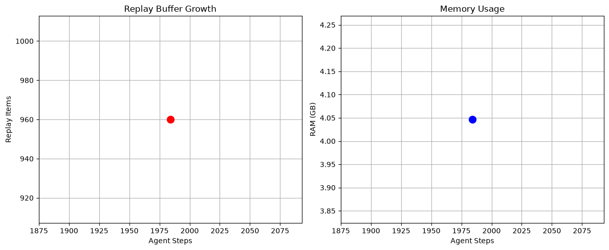 Figure: Example training log visualization. Left: replay buffer growth. Right: memory usage. Data points from actual training runs.
Note: During early training (first ~2,000 steps), the replay buffer is still filling, so metrics won’t be written yet. You need enough steps to complete the first episode before scores.jsonl will have data. The Cartpole Balance task typically requires several thousand to tens of thousands of steps to complete its first episode.
Advanced: Observing the World Model’s “Imagination”
This article’s title mentions “world models,” but so far we’ve mainly been looking at policy training. The world model’s most core capability is actually imagination — given the current state and an action, predicting what will happen in the future. DreamerV3’s policy is trained in imagined space, so understanding this capability is essential.
What Is “Imagination”
In DreamerV3, “imagination” specifically means: the RSSM starts from the current latent state and, without interacting with the real environment, autonomously rolls out multiple future steps. At each step, the RSSM outputs:
- Next latent state: The encoded future state
- Predicted observation: The reconstructed frame through the decoder (64x64 pixels)
- Predicted reward: The estimated immediate reward
- Predicted termination: Whether the episode has ended
This process happens entirely within the model, with no real environment interaction needed. The Actor-Critic policy is trained in this imagined space — the Actor selects actions and the Critic evaluates values, all within the “mind.”
How to Observe Imagination Quality
The most intuitive approach is to compare imagined frames with real frames. Here’s how:
- Collect a trajectory from the real environment (e.g., 100 steps)
- Use the RSSM encoder to encode the first observation, obtaining the initial latent state
- Starting from the second step, use real actions to drive the RSSM rollout (teacher forcing)
- At each step, use the decoder to reconstruct frames and compare with real frames
If the world model has learned well, the reconstructed frames should be very close to the real frames. As the number of rollout steps increases, error will gradually accumulate and frames may become blurry — this is normal.
Implementation in Code
Here is a simplified rollout analysis script showing how to load a trained model and perform imagination rollout:
import pickle
import numpy as np
import matplotlib.pyplot as plt

# Load trained checkpoint
with open('~/logdir/wm_cartpole_balance/ckpt/latest/agent.pkl', 'rb') as f:
    agent = pickle.load(f)

# Sample a real trajectory from the replay buffer
# (actual implementation needs replay buffer access — simplified here)
real_obs = sample_trajectory(length=100)  # shape: (100, 64, 64, 3)

# Encode the first observation
latent = agent.dynamics.encoder(real_obs[0])

# Drive rollout with real actions (teacher forcing)
reconstructed = []
for t in range(1, 100):
    action = real_actions[t-1]  # real action
    latent, _ = agent.dynamics.transition(latent, action)
    pred_obs = agent.dynamics.decoder(latent)
    reconstructed.append(pred_obs)

# Compare reconstructed and real frames
fig, axes = plt.subplots(2, 5, figsize=(15, 6))
for i in range(5):
    idx = i * 20  # look at a frame every 20 steps
    axes[0, i].imshow(real_obs[idx])
    axes[0, i].set_title(f'Real t={idx}')
    axes[0, i].axis('off')
    axes[1, i].imshow(reconstructed[idx-1])
    axes[1, i].set_title(f'Reconstructed t={idx}')
    axes[1, i].axis('off')

plt.tight_layout()
plt.savefig('imagination_comparison.png')
plt.show()
How to Judge Imagination Quality
When examining the comparison charts, focus on these aspects:
- Short-term prediction (1–10 steps): Reconstructed frames should be nearly identical to real frames. If there’s a large gap, the model hasn’t learned well yet
- Medium-term prediction (10–50 steps): Frames may start to blur, but the overall structure should be preserved (e.g., the cartpole’s pole is still there, position is roughly correct)
- Long-term prediction (50+ steps): Frames may be severely distorted — this is normal, as errors accumulate
Another criterion is policy performance in imagined space. If the Actor’s policy trained in imagined space also works when deployed in the real environment, the imagination quality is good enough. Conversely, if the policy performs poorly in the real environment, the imagined space may be too far from reality.
Imagination-Space Evaluation Metrics
In metrics.jsonl, you can monitor these imagination-related metrics (key names may vary by version):
train/loss/dyn: World model dynamics prediction loss — decreasing means prediction ability is improvingtrain/loss/dec: Decoder reconstruction loss — decreasing means frame reconstruction quality is improvingtrain/loss/rew: Reward prediction loss — decreasing means reward predictions are more accurate
These losses decreasing is a necessary but not sufficient condition — low reconstruction error doesn’t guarantee a good control policy. Ultimately, you need to check whether the episode return in scores.jsonl is increasing.
Step 6: Understanding Training Output
After training completes, the directory structure under logdir looks like this (verified with commit e3f02248):
~/logdir/wm_cartpole_balance/
-- config.yaml               # Training config (complete hyperparameter record)
-- metrics.jsonl             # Training metrics (JSON Lines format, one line per ~2000 steps)
-- scores.jsonl              # Episode scores (JSON Lines format, one line per completed episode)
-- ckpt/                     # Model checkpoints
|   -- latest                # Latest checkpoint path
|   -- 20260804T194935F161160/
|       -- step.pkl          # Training step count
|       -- agent.pkl         # Model weights (approximately 2GB)
|       -- replay.pkl        # Replay buffer state
|       -- done              # Save completion marker
-- replay/                   # Replay buffer data
-- scope/                    # Performance monitoring metrics
    -- fps-train.float       # Training FPS
    -- fps-policy.float      # Policy FPS
    -- replay-*.float        # Replay buffer statistics
    -- usage-psutil-*.float  # System resource usage (CPU/memory)
Key file descriptions:
- metrics.jsonl: Contains replay buffer status, FPS, memory usage, and other training metrics. Each line is a JSON object with keys like
replay/items,fps/policy,usage/psutil/proc_ram_gb, etc. - scores.jsonl: Records each episode’s score and length. Only has data after enough steps to complete the first episode
- ckpt/agent.pkl: Model weights file, usable for resuming training or inference. Note that a single checkpoint is approximately 2GB
- scope/: Binary-format performance metrics, readable with Python to analyze training efficiency
Analyze training results with Python:
import json
import matplotlib.pyplot as plt

# Read metrics.jsonl
with open('~/logdir/wm_cartpole_balance/metrics.jsonl') as f:
    metrics = [json.loads(line) for line in f]

# Print all metric keys
print('Metric keys:', list(metrics[0].keys()) if metrics else 'No data')

# Plot replay buffer growth
steps = [m['step'] for m in metrics]
items = [m.get('replay/items', 0) for m in metrics]

plt.figure(figsize=(10, 5))
plt.plot(steps, items)
plt.xlabel('Agent Steps')
plt.ylabel('Replay Items')
plt.title('DreamerV3 Training Progress')
plt.savefig('training_progress.png')
plt.show()

# Read scores.jsonl (if data exists)
try:
    with open('~/logdir/wm_cartpole_balance/scores.jsonl') as f:
        scores = [json.loads(line) for line in f]
    if scores:
        print(f'Completed {len(scores)} episodes')
        print('Last episode:', scores[-1])

        plt.figure(figsize=(10, 5))
        plt.plot([s.get('step', i) for i, s in enumerate(scores)],
                 [s.get('score', 0) for s in scores])
        plt.xlabel('Step')
        plt.ylabel('Episode Score')
        plt.title('Episode Returns')
        plt.savefig('episode_scores.png')
        plt.show()
    else:
        print('scores.jsonl is empty — more training steps needed')
except FileNotFoundError:
    print('scores.jsonl does not exist')
Troubleshooting Common Issues
Issue 1: MuJoCo rendering error “GLFW error”
This is usually caused by not configuring the rendering backend correctly. If you’re on a remote server or headless machine, set the environment variable to use offscreen rendering:
export MUJOCO_GL=egl   # With GPU
# or
export MUJOCO_GL=osmesa  # Without GPU
Issue 2: DreamerV3 training is very slow
Several possible causes: no GPU (pure CPU training is 10x+ slower), batch size too large (try reducing it), not enough environment parallelism. If you have a GPU, confirm JAX correctly recognizes CUDA (check with jax.devices()).
Issue 3: Training reward not increasing
Could be an unsuitable learning rate, task too difficult, or not enough training steps. Try switching to a simpler task first (e.g., a reach task) to verify the pipeline, then move to harder tasks. DreamerV3’s default hyperparameters are tuned for most MuJoCo tasks and generally don’t need modification.
Issue 4: Out of memory (OOM)
DreamerV3 needs to store a replay buffer. If memory is insufficient, reduce the buffer size. Modify buffer_size=1e5 in the configs (the default is larger).
Issue 5: Process killed (OOM Killer)
If training runs for a while and then suddenly gets killed by the system (terminal shows “Killed”), the Linux OOM Killer was likely triggered. This typically happens during JAX compilation or replay buffer filling, when memory usage spikes briefly. Solutions:
# Check system memory
free -h

# If memory is insufficient, you can:
# 1. Reduce replay buffer size (override in configs.yaml or command line)
python dreamerv3/main.py --replay.size 1e5 ...

# 2. Increase swap space (temporary fix)
sudo fallocate -l 8G /swapfile
sudo chmod 600 /swapfile
sudo mkswap /swapfile
sudo swapon /swapfile

# 3. Use a smaller batch size
python dreamerv3/main.py --batch_size 8 ...
At least 32GB of memory is recommended for running DreamerV3. If running in a VM, make sure enough memory is allocated.
Issue 6: JAX throws AssertionError (no-GPU environments)
If your machine doesn’t have an NVIDIA GPU, you may encounter an AssertionError in jax/_src/xla_bridge.py when running training. This is because configs.yaml defaults the JAX platform to cuda, and JAX crashes when it can’t find a GPU backend. The fix is to add --jax.platform cpu to the command line:
python dreamerv3/main.py \
  --configs defaults dmc_vision \
  --task dmc_cartpole_balance \
  --jax.platform cpu
This overrides the default in the config file, forcing JAX to use the CPU backend. GPU users don’t need this parameter.
Next Steps: From MuJoCo to Isaac Sim
MuJoCo is great for quick algorithm validation, but its rendering fidelity is limited. If you need more realistic visual input (e.g., training a robot to recognize objects from camera images), you can upgrade to NVIDIA Isaac Sim.
Isaac Sim is built on the Omniverse platform, offering physically accurate simulation and high-fidelity rendering. Its API differs from MuJoCo, but DreamerV3’s training pipeline is the same. However, migrating from MuJoCo to Isaac Sim isn’t as simple as writing an environment wrapper. Differences you’ll need to handle include:
- Observation Design: Isaac Sim’s visual output format, resolution, and camera parameters differ from MuJoCo and need re-adaptation
- Camera Latency: High-fidelity rendering introduces additional latency, which may affect training stability
- Physics Timestep: The two engines differ in simulation frequency and integration accuracy; action repeat may need adjustment
- Action Scaling: The range and meaning of the action space may differ and need recalibration
- Domain Randomization: Sim-to-Real transfer requires redesigning the randomization strategy
I’ll write a separate article on this advanced topic later. For now, the most important thing is to get MuJoCo + DreamerV3 running and understand the world model training pipeline.
Optional: One-Click Docker Deployment
If you’ve spent too much time on local environment setup (CUDA versions, MuJoCo rendering, JAX GPU, etc.), consider using Docker for environment consistency. Here’s a basic Dockerfile example:
FROM nvidia/cuda:12.2.0-runtime-ubuntu22.04

RUN apt-get update && apt-get install -y \
    python3.11 python3-pip libosmesa6-dev \
    libgl1-mesa-glx libglfw3-dev

WORKDIR /app
COPY requirements.txt .

# Filter out ale_py (delisted) and autorom
RUN grep -v "ale_py" requirements.txt | grep -v "autorom" | pip install --no-cache-dir -r /dev/stdin
RUN pip install "jax[cuda12]" mujoco dm-control

COPY . .

# Default to CPU mode; remove --jax.platform cpu when GPU is available
CMD ["python", "dreamerv3/main.py", \
     "--logdir", "/app/logdir", \
     "--configs", "defaults", "dmc_vision", \
     "--task", "dmc_cartpole_balance", \
     "--run.steps", "1e6", \
     "--jax.platform", "cpu"]
Build and run:
# Build image
docker build -t dreamerv3 .

# Run (mount log directory to host)
docker run --gpus all -v $(pwd)/logdir:/app/logdir dreamerv3

# If CPU only, remove --gpus all
docker run -v $(pwd)/logdir:/app/logdir dreamerv3
Memory note: Docker containers can by default use all host memory, but if you’re using Docker Desktop (macOS/Windows), you need to allocate at least 32GB in settings, or training inside the container will be OOM-killed.
The advantage of Docker is that the environment is fully reproducible — no more “it works on my machine” problems due to system differences. This is especially useful for team collaboration and reproducing paper experiments.
Summary
Today we built a complete world model experimentation environment: MuJoCo handles physics simulation, DreamerV3 handles world model training. We learned how to view and analyze training logs (metrics.jsonl and scores.jsonl) and plot training curves with Python. The entire process from installation to running the first experiment takes about 30 minutes to an hour (depending on network speed and whether you use Docker).
Once it’s running, you can try:
- Progressively increasing task difficulty (walker stand -> cheetah run -> walker walk -> humanoid walk)
- Running imagination rollouts to observe the world model’s “imagination” quality
- Adjusting hyperparameters and observing changes in imagination-space quality
- Comparing DreamerV3’s sample efficiency with traditional RL (e.g., PPO)
- Adding language conditioning to the world model to explore language grounding possibilities
Practice yields true understanding. After running experiments once, your understanding of world models will be deeper than from reading ten papers.
In the next article, I plan to discuss a more cutting-edge topic: how to use world models to generate synthetic data for augmenting VLA training. This is a hot direction in the convergence of VLAs and world models — stay tuned.
Comments